Excel Budget: Calculations

In this task, you will complete the following objectives:

Open and existing file and rename it
Substitute the amounts in the original files, adding decimals
Change the decimal options
Enter formulas to automatically add totals
Extend the formulas
Enter Average formulas and extend them
Add a new row with new information
Complete a reading challenge
Create a pie chart with your information
Create your own budget for four months, adding average and totals formulas, and a pie chart

You will evaluate yourself (compete rubrics) at the end. Click on the arrow to read the rubric (evaluation) items at the end.
(To come back here, click the BACK button on your browser.)

In the first Web Task in the Excel series, you learned how to open the program, use the common menu options and shortcuts, enter and format text in cells, and change cell sizes.

You entered the following information in the first part.

	January	February	March
Rent	303.00	303.00	303.00
Car Payment	249.00	249.00	249.00
Gas Bill	75.00	92.00	87.00
Electricity Bill	45.00	32.00	40.00
Water Bill	20.00	20.00	28.00

To begin this exercise, we are going to add decimals to the numbers in each item and learn to work with them.

Activity 1: In the Excel sheet that you saved from your first Task, substitute the following dollar amounts in each cell.

	January	February	March
Rent	903.41	903.41	903.41
Mortgage	903.41	903.41	903.41
Car Payment	449.27	449.27	449.27
Gas Bill	125.32	115.67	95.99
Electricity Bill	45.64	22.92	40.22
Water Bill	20.88	20.24	28.89

-->>Save your spreadsheet as "your initials budget2." You now have two Excel Spreadsheets: budget1 and budget2. This Task will be saved as "budget2."

NOTE: If you don't see a button that you want to use, click on the small Down Arrow images you will find on your toolbar. Those show you the hidden options on your toolbar that don't fit the screen.

Finding a Sum (Adding)

Activity 2

Select cell A10. Type the word Total in the cell. Move to cell B10. This cell will show the total amount paid in January for the five categories.

There are several ways to have Excel calculate the sum (total) of the values (amounts) in cells B3 through B7. One method is to type the following in cell B10: =B3+B4+B5+B6+B7. (Try it, if you want. Then erase the total and use the next way).

However, there is a better method. Select cell B10. Click on the AutoSum button on the Standard Toolbar. The AutoSum button shows an uppercase sigma (see image).

A box appears around cells B3 through B9. Use your mouse to select only cells B3 though B7, then press Enter on your keyboard. Use the automatic copy feature to calculate the sums in the rest of the columns.

Hint: Click on B10 and drag to M10. This copies the formula!

-->>Save your spreadsheet.

Finding an Average

Activity 3

An average shows the total sum of several values (amounts) divided by the number of items included to reach the total.

For example, imagine that when you were in school, you got six grades in your art class: 97, 89, 91, 100, 94, and 100. To find out your grade average in your class, you would first add all of the values or amounts:

100

100
_________

Total: 572

Next, you would divide that total by the number of grades you added.

572 � 2 = 95.3333 Rounded off to 95. Your average in Art would be 95.

Now we'll let Excel figure our our average expenses.

In cells O3 through O7, you want to find the average paid for each bill for each month. Again, there are several ways to do this. The method we will use is the Paste Function feature.

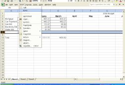
Select cell O2. Type Average. Select cell O3.

Click on the Insert Function button (Excel XP) or the Paste Function button (Excel 2000).

This action lets you to choose a math function to enter in a cell. Select the function Average from the right-hand column, as shown in the image.

Click OK. A dialog box appears. The automatic setting should be B3:N3, indicating Excel will find the average of cells B3 through N3 (Notice that the colon (:) stands for "through."

Click in this space and change the N3 to M3 (B3:M3) since we do not want the empty cell N3 to be included in the average.

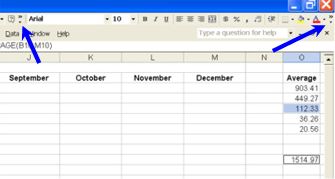
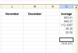
Click OK. Use the automatic copy feature to place averages in cells O4 through O10.

Column O in your spreadsheet should look like the model at the right

Note: The information #DIV/0! in O8 and O9 indicates division by 0 is undefined. I would delete those.

-->>Save your spreadsheet.

Inserting Rows & Columns

Activity 5

Suppose you want to add another bill to your budget - your MasterCard Bill for instance. There is space in rows 8 and 9 for more data (information); however, to keep a space between the data and the totals, you decide to insert a new row. To do this, select row 8 by clicking on the 8 at the far left of the screen. Select Insert | Rows. A new row is added.

NOTE: New rows are added above the selected row. New columns are added to the left of a selected column.

Go ahead and add the MasterCard Bill. Oops! The text is too big for the column. How can you make the column fit the text? If you need to review, go back to the your first budget Web Task and practice changing cell widths.

-->> Save your spreadsheet.

Manipulating Borders

Activity 6

Before printing a spreadsheet, you may want to place borders around some or all of the cells. (The default (factory/automatic) setting in Excel 2000/XP includes no borders around any cells.)

Highlight cells A1 through O12. Select Format | Cells. Click on the Borders tab. In the dialog box, you can select borders around the entire selected area, around each cell, or only along certain edges.

Place a border around the A1:O12 block, around individual cells. Click OK.

To view how the spreadsheet will look when printed, click on the Print Preview button on the Standard Toolbar. Notice that the border appears only around the outside, as you told it to do . However, that the budget does not fit on a single sheet of paper. To go back to your other view, click on the Close tab.

-->> Save your spreadsheet.

Using Charts

Activity 8

Highlight cells A3 through D8. Click on the Chart Wizard button in the Toolbar. Select Pie from the chart options on the left. Click Next until you see a box to name your chart. Name the Chart 2004 Budget and click Next and OK to accept all defaults (basic settings). Click Finish to complete the chart of your budget. Your pie chart appears on your Excel spreadsheet. A picture is worth a thousand words!

-->> Print your spreadsheet, sign it, and place it in your folder.

Activity 9

Click on the arrow to complete the Reading Challenge.

Activity 10

PROJECT: Using all of the tools you learned, create your own budget for four months. Add the totals for each month and print a pie chart to compare amounts.

Print your budget spreadsheet, sign it, and place it in your folder.